Revista IECOS, 25(2), 35-52 | Julio-Diciembre 2024 | ISSN  2961-2845 | e-ISSN  2788-7480

EFFECTS OF COPPER PRICES VOLATILITY ON PERUVIAN ECONOMICS: EMPIRICAL EVIDENCE FROM TVP-VAR-SV MODELS

EFECTOS DE LA VOLATILIDAD DE LOS PRECIOS DEL COBRE EN LA ECONOMÍA PERUANA: EVIDENCIA EMPÍRICA A PARTIR DE MODELOS TVP-VAR-SV

Jose Carlos Muñoz Aguilar

Centro de Investigaciones Académicas, Lima, Perú

E-mail: jose.munoz.a@uni.pe

https://orcid.org/0000-0002-1090-6012

https://doi.org/10.21754/iecos.v25i2.2195

Recibido (Received): 24/03/2024 Aceptado (Accepted): 11/06/2024 Publicado (Published): 27/09/2024

ABSTRACT

Considering the strong performance of copper prices in the past few years and the dependence on this mineral for Peru, this research was developed. with the objective to analyze the effects of copper prices volatility on these main macroeconomic variables. For this are proposed a TVP-VAR-SV model. The results indicate that a 1% rise in copper prices leads to a corresponding increase of 0.03% in GDP growth, an increases of 3.77% in exports and a decrease of 1.22% in exchange rate, on average, within the first quarter following the price change. However, it can be seen how the effects are amplified in periods of high volatility in the price of copper. In 2009Q4, these effects are amplified, where the GDP increases by 0.69%, exports increase by 5.86% and the exchange rate decreases up to 1.69%.

Keywords: TlVP-VAR-SV, Copper Price, GDP, Exports, Exchange Rate.

JEL Classification: C32, C55, Q33.

RESUMEN

Dado un contexto de altos precios del cobre en los últimos años y la dependencia de este mineral para el Perú, se desarrolló esta investigación. con el objetivo de analizar los efectos de la volatilidad de los precios del cobre sobre estas principales variables macroeconómicas. Para ello se propone un modelo TVP-VAR-SV. Los resultados indican que ante un incremento de 1% en el precio del cobre, en promedio el crecimiento del PBI aumenta en 0.03%, las exportaciones aumentan en 3.77% y el tipo de cambio disminuye en 1.22% en el primer trimestre del shock, a través del período de estudio. No obstante, se observa cómo los efectos se amplifican en periodos de alta volatilidad en el precio del cobre. En 2009T4, estos efectos se amplifican, donde el PIB aumenta un 0.69%, las exportaciones aumentan en 5.86% y el tipo de cambio disminuye hasta un 1.69%.

Palabras clave: TVP-VAR-SV, Precio del Cobre, PIB, Exportaciones, Tipo de Cambio.

1. INTRODUCTION

The Peruvian economy is one of the main copper producers in the world, being this commodity, the most important mineral in the country, since it sustains a large part of its economic growth to mining extraction, mainly copper. Since the mid-1990s, Latin America has remained the main destination for mining investments globally. According to the United States Geological Survey (USGS), Peru is the second largest copper producer globally, behind Chile, and the third country with the largest copper reserves in the world, only surpassed by Chile and Australia (Rodriguez et al., 2019; Pedersen, 2019).

However, the prices of commodities, especially copper, present a high and frequent variability, which could have repercussions on the main macroeconomic variables given that it is an economy whose exports they depend on this mineral (Rodríguez et al., 2019). By the year 2021, copper represented 52.5% of the metal mining GDP, followed by gold that represented 25.5%, zinc with 6.6%, iron with 5.6%, lead with 4.8%, among other minerals produced by the Peru (Ministry of Energy and Mines, 2022).  Therefore, faced with this problem of overdependence on copper for the Peruvian economy, we can ask ourselves: How do changes in the price of copper affect the main macroeconomic variables of Peru? especially in these current periods of great price volatility of said metal.

To address this type of inquiry, the literature presents studies on the response of key macroeconomic variables to fluctuations using Vector Autoregressive (VAR) models. Studies such as Rodriguez et al. (2019) specify that Peru is a developing country that depends on commodities, so it would be subject to mineral exports; and this would be vulnerable to negative shocks of prices and  volatility.  Likewise, the literature has focused its interest on studying the impacts of commodity price variations on the economic behavior of different countries, especially countries with a high dependence on these minerals. Authors such as Medina (2010), Naranpanawa & Bandara (2012), Gondo & Perez (2018), Pedersen (2019), Rodríguez et al. (2019), Urbina & Rodríguez (2023), and Cornejo et al. (2022), focused their studies on empirically studying the impacts of comlmodity prices on the main economic variables (gross domestic product, inflation, level of exports, exchange rate, etc.) of the different countries in the region, which in general show that a commodity price shock generates an acceleration in the growth of the economy. The main methodology used in this line of research was the Autoregressive Vector models with constant parameters (CVAR).

Medina (2010) studied how these fluctuations in commodity prices impact the fiscal position of the countries, and for this he used a VAR model with Cholesky identification, with which he concluded that the Latin American countries analyzed have been applying efficient fiscal rules. Likewise, Gondo & Perez (2018), for their part, estimated, utilizing a Bayesian Hierarchical Panel VAR model with sign restrictions, the dynamic impacts of commodity and oil price fluctuations on macroeconomic and financial variables of Latin American countries. For which they used a price index of all commodities, finding that a positive shock to comlmodity prices generates an expansion of economic real sector with certain heterogeneity where growth was greater in Peru and Colombia compared to Chile and Mexico.

Pedersen (2019) studied the heterogeneity of the impacts of the copper price shock on the Chilean economy, depending on the source of the shock, using a sign-restricted SVAR model, where he found that the impacts of the copper price demand shock imply greater growth in Chile, while the effects of the copper supply shock are, at least in the short term, negative for Chilean growth. For their part, Rodríguez et al. (2019) analyzed how copper price shocks are related to the main macroeconomic variables of Peru, using a Vector Autoregressive (VAR) model, finding that a copper price shock accelerates growth. of GDP by 0.3% until the second quarter and then diluted until the fifth quarter.

With which there is enough literature on these effects of commodity prices on the Peruvian economy, this effect being homogeneous for all analysis periods. However, these effects may have varied in recent years, given the great volatility of the price of commodities and stressful events for developing economies, such as the international financial crisis. Therefore, this research aims to determine the effects of a copper price shock on the key macroeconomic variables in a small and open economy dependent on the export of said mineral, such as Peru; and how these effects vary over time in which various episodes of stress have arisen for the Peruvian economy.

So, this work makes two contributions. First, determine the effects of the copper price on the key macroeconomic variables of Peru such as GDP, Inflation, Exchange Rate and Interest Rate. Second, determine the heterogeneity of these effects over time. For which it uses a TlVP-VAR-SV model to be analyzing the effects of copper price volatility on key macroeconomic variables. This type of model, compared to a standard VAR, allows capturing the effects of the abrupt and progressive changes that the Peruvian economy suffered during the period of analysis, in the face of structural reforms, changes in economic policy and external shocks, as pointed out by Calero & Salcedo (2021), and also allows us to capture the heteroskedasticity of the shocks to which a small and open economy like the Peruvian one is exposed, as specified by Urbina & Rodríguez (2023).

The present work contrasts the hypothesis that there are heterogeneous effects of copper price shocks on macroeconomic variables. Finding what in the face of a 1% rise in copper prices leads to a corresponding increase of 0.03% in GDP growth, an increases of 3.77% in exports and a decrease of 1.22% in exchange rate, on average, within the first quarter following the price change, however, it can be seen how the effects are amplified in periods of high volatility in the price of copper, where the GDP increases by 0.69%, exports increases in 5.86% and the exchange rate decreases up to 1.69%.

These results will serve as inputs for future economic policies that could help counteract these effects and thereby promote sustained economic growth that materializes in economic and social development, specifically in regions where extractive activities for said mineral are carried out. The remainder of this paper is organized as follows. Section 2 describes the methodology used. Section 3 describes the data used as well as the source from which it was obtained. Section 4 presents an empirical result. Section 5 conclude

2. METHODOLOGY

2.1 TVP-VAR-SV frameworks

To determine the effects of the copper price on the key macroeconomic variables of Peru, a Vector Autoregressive (VAR) model will be used with different specifications associated with the dynamics of its parameters. Followed those proposed by Urbina & Rodríguez (2023), Chan & Eisenstat (2018) and Primiceri (2005), who propose a VAR model with parameters that change over time and with stochastic volatility (TlVP-VAR-SV):

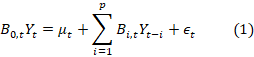
where B_0,t is the conltemporaneous effects matrix with onles on the diagonall, Y_t is the vector of observable endogenous variables that will be inserted into the model (Copper Price, GDP, Inflation, Exchange Rate, Interest Rate), μ_t is the vector of time-changing intercepts,  B_i,t is the vector of lparameters of the llagged variables, andl  is the vector of heteroskedastic unobservable shocks such lthat ς_t~N (l0, Σ_t). Here the variance and covariance matrix is a diagonal matrix

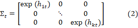
Assuming that the llog vollatilities folllow a randlom walk process h_i,t = h_i,t-1+ς_i,t , for all i = 1,2,3,…k; such that  ς_t~N (l0, Σ_h) and the ilnitial condition h₀ is a parameter to estimate. Urbina & Rodríguez (2023) propose two groups of parameters that change over time to be estimated. The first group is the vector of intercept and lags of the coefficients of the variables β_t changing over time. The lsecond lgroup is lthe vector lof lcoefficients of lcontemporaneous effects changing in time γ_t, where β_t = vec( (u_t,β_1t,…,β_pt )´ ) , vector of dimensions k_β*1, where  k_β=n(np+1); and , vector of dimensions k_γ*1,, where  k_γ=n(n-1)/2.

The dynamics of the time valrying parameters within the model can be specified as follows:

So, Equation (1) can be written in the following way  . Where   and W_t is a llower ltriangular matrix of contemporaneous effect coefficients, with dimension n*k_γ. With this, the model can be formulated as a statel-space model: y_t=X_t θ_t + ϵ_t, where ; θ_t = θ_t-1 + η_t, where θ_t = (β'_t, γ'_t)', with dimensionl k_θ = k_β + k_γ, and the initial condition θ₀ is estimated, assuming η_t ~ N ( 0, ∑_θ).

According to Urbina & Rodríguez (2023) the best VAR model that adjusts to the reality of Peruvian economic activity is with stochastic volatility because it allows capturing the heteroscedasticity of the shocks to which a small and open economy like Peru is exposed. Likewise, a TlVP-VAR-SV model alllows the contemporaneous parameters and those associated with the lagged variables, intercept and variance of the errors to change over time. Being able to capture the effects of the abrupt and progressive changes that the Peruvian economy suffered during the analysis period, in the face of structural reforms, changes in economic policy and external shocks, as indicated by Calero & Salcedo (2021).

The estimation of the model was carried out following what was proposed by Urbina & Rodríguez (2023), who estimated the model by the Bayesian method using the lprecision sample of Chanl & Jleliazkov (200l9). Therefore, the Giblbs sampling algoritlhm uses the precision sample of Clhan & Jleliazkov (2009). Likewise, the initial conditions of the priors folllow a normall distrilbution such that θ₀ ~ N (a_θ,V_θ) y h₀ ~ N (a_h,V_h ), in agreement with Chan & Eisenstat (2018) y Urbina & Rodríguez (2023). Where the hyperparameters are: a_θ = 0 and V_h = 10 * I_n, Assuming that the mean of the prior  is 0.12, the mean of the prior  is 0.01² or the VAR coefficients and 0.1² for the intercept.

Likewise, the identification of the proposed model was developed through recursive Cholesky identification; Therefore, we use the triangular decomposition of the error variance and covariance matrix.

which represents the set of endogenous variables, organized from the most exogenous variable to the least exogenous. Where y_1t is the price of copper, y_2t is the exchange rate, y_3t   is the reference interest rate, y_4t   is inflation, y_5t is exports, and y_6t is GDP. This arrangement follows what was proposed by Urbina & Rodríguez (2023) and Kumah & Matovu (2007) who consider that comlmodity prices are the most exogenous variable, since it is determined at the internationall level, and Peru is a country and a small economy and open to the world, which has no influence on the price of said commodity.

3. DATA

The data as macroeconomic variables, GDP (Quarterly frequency), Inflation (monthly frequency), Exchange Rate (daily frequency) and Reference Interest rate was obtained from the official institution as BCRP, where all variables were transformed to quarterly frequency. The data was analyzed in the time period from 2001 to 2019.

After collecting the data, a univariate analysis of seasonality was carried out, seasonally adjusted if necessary, using statistical techniques, to later determine if the variables are stationary. Once the seasonality and stationarity requirements were met, the econometric models were proposed.

4. EMPIRICAL RESULTS

According to the proposed TlVP-VAR-SV model, it founded that the paralmeters aslsociated with the contemporary and the lags of effects of the copper price, GDP, exports, inflation, exchange rate, interest rate, show intense variations over time. The intercepts have a notable variation over time.

In the analysis of the response impulse functions, Figure 1 shows the reslponses of the variables to a copper price shock in three dimensions: on the x-axis the percentage of deviation, on the y-axis the periods after the shock occurred, and on the z-axis, how these responses vary over the years. A copper price shock would not generate a significant response in the very short term in GDP (first quarter after the shock occurred). Then for the following periods, the effect is heterogeneous. The first years of analysis (2001 - 2010), which would reflect the period of commodity price super cycle, the effect of a copper price shock becomes positive. For the second section of the analyzed period (2011 - 2019), a negative response was observed, a period influenced by the start of tapering in 2013, Chinese stock market correction (2015 - 2016), trade war between the US and China (2018 - 2019). These results follow the line of what was stated by Urbina & Rodríguez (2023) who point out that in the face of a mineral and metal price shock there is a positive response of GDP and mining exports, varying over time and reaching a peak around 2009.

Likewise, it is observed that exports have a positive response in the short term throughout the analyzed period, given that 60% of total exports are mining exports, and a positive shock to the price of Peru's main mineral would generate an increase in value of exports. Exports would be the transmission mechanisms of a copper price shock to GDP. Also, a negative response of the exchange rate to a copper price shock is evident in all periods of time with certain fluctuations, it peaks in mid-2010. The interest rate and inflation have a negative response to a shock. of the price of copper, in the very short term, then that effect fades.

Also, the figure 1 shows the evolution over time of the median responses of the variables GDP, exports, inflation, exchange rate, interest rate to a copper price shock. The GDP growth increases by 0.03%, given a 1% increase in the price of copper. This increase in GDP would be generated by a higher value of traditional GDP, specifically the value of mining exports, where copper is a predominant factor, which generates GDP growth above its potential in the short term. This result follows the line of what was indicated by Urbina & Rodríguez (2023) and Rodríguez et al. (2019). Exports increased by 3.77%, given a 1% increase in the price of copper, the first quarter after the shock. After the shock, the effect decreased until it disappeared in the fifth period. This effect is generated due to the great dependence on minerals, particularly copper, in Peru's total exports.

The exchange rate reacts negatively during the first four quarters after the copper price shock, after which the impacts become insignificant. Given a 1% increase in the price of copper, in the very short term (first quarter after the shock), the exchange rate decreases by 1.22%. It being understood that the copper price shock would generate a greater flow of capital entering the Peruvian economy, evidenced in the increase in the value of mining exports, causing the appreciation of the local currency, and thereby putting pressure on the drop in the exchange rate. These unexpected income from greater resources reduce the exchange rate, making exports more expensive, causing a decrease in the economy's competitiveness. The interest rate and inflation have a negative reaction in the first quarters after the copper price shock, but this is not statistically significant.

Figure 1

RIF a shock of the price of copper

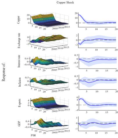
Note. The left column shows the responses of the variables to a copper price shock in three dimensions: on the x-axis the percentage of deviation, on the y-axis the periods after the shock occurred, and on the z-axis, how these responses vary over the years. On the other hand, in the left column shows the median of all the impulse response functions throughout the analysis period.

Figure 2 shows the responses of the various analysis variables to a copper price shock for specific periods (eg 2008q4, 2009q4, 2014q1). In the 2008q4 period it was evident that global activity registered a strong contraction, linked to a significant drop in global demand, affecting in a synchronized manner different international markets, where the raw materials market was not the exception. For the 2009q4 period, there was a rapid recovery in the prices of raw materials hand in hand with signs of recovery in global activity and improvements in perception of risk by global financial markets generated by large bailouts from the FEFD. Both periods show the periods with the greatest volatility in the price of copper during the analysis period. And the 2016q2 period was recorded as one of the periods with the lowest volatilities in the price of copper.

The impulse response functions associated with the 2008q4 period show that GDP increases 0.69% until 3rd quarter, the exchange rate responds decreasing in 1.91% until 2nd quarters, the exports increase in 5.64% until 2nd quarters and Inflation and the interest rate did not have a significant response. Likewise, the impulse-response functions associated with the 2009q4 period show that, that GDP increases 0.68% until 3rd quarter. The exchange rate responds decreasing in 1.95% until 2nd quarters. The exports respond increases 5.86% until 2nd quarters. The inflation and the interest rate did not have a significant response

The GDP responds with an increase in subsequent periods through the short-term increase in exports. The exchange rate responds with a significant decrease in the first two quarters, and then the effect decreases, this is related to the appreciation of the local currency supported by the healthy economy of that period despite the financial crisis. Inflation also reacted negatively, thanks to the intervention on inflationary pressures by the BCRP in the face of great growth in the Peruvian economy. On the other hand, the responses associated with 2016q2 showed that the GDP response to a copper price shock was slightly positive, in 0.19% until 3rd quarter, the exchange rate decreasing in 1.71% until 2nd quarters, and the exports increase in 4.96% until 2nd quarters.

Likewise, we can observe that the impulse response functions of a standard VAR model without changing parameters in over time, resembles the results of periods of high copper price volatility (2008q4 and 2009q4), showing that it captures these high volatilities in its dynamics, but without being able to distinguish these periods with others of less volatility.

Figure 2

RIF a shock of the price of copper per specific years

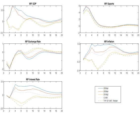
Note. The FIRs are shown according to years of high and low volatility of the copper price. The blue lines represent the FIRs of 2008q4, the red lines represent the FIRs of 2009q4, the yellow lines represent the FIRs of 2016q2, the purple dotted lines represent the FIRs of a CVAR, and the green dashed lines represent the median of the FIRs of a TVP-VAR-SV.

On the other hand, Table 1 shows the evolution and importance of a copper price shock on the variability of the macroeconomic variables studied. Where the shock to the price of copper explains 37.48% of the variability of GDP, evidencing the great importance of this commodity for the Peruvian economy, especially the mining sector; also explains 38.03% of the variability of the Exchange Rate, reflecting the vulnerability of the Peruvian economy to exports from the mining sector; and explains 47.69% and 49.74% of the variability of inflation and the interest rate, respectively.

Tabla 1

Decomposition of the variance before a shock of the price of copper

Horizon	GDP	Exports	Exchange rate		Inflation	Interest rate
1	0.70	46.78	18.29	5.23		0.91
2	7.1	58.42	31.09	10.98		9.30
3	12.23	59.71	31.92	20.24		17.98
14	36.02	59.71	37.09	47.17		44.93
	37.48	59.71	38.03		47.69	49.74

Note. The variability of each variable is shown, and the importance of the copper price shock on that variability.

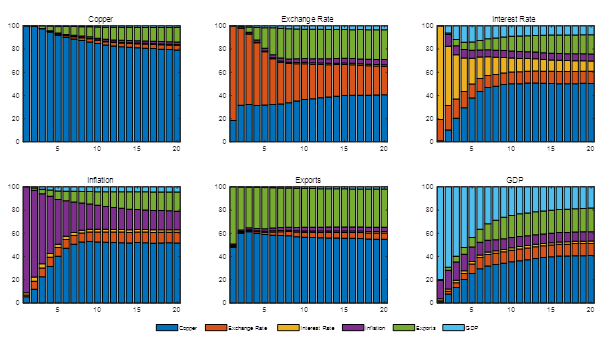
Figure 3 shows the historical breakdown of the variance of the macroeconomic variables studied in this paper. The contribution of a copper price shock to GDP growth fluctuations shows that in the first periods of time studied (year 2002) the contribution is very slightly indirect and not significant. From the year 2003 to the year 2013 (period of time where the super cycle of precise commodities was evidenced) a notable growth of the GDP is reflected, substantially explained by a shock of the price of copper, evidencing a direct relationship between both variables and a high correlation of copper with the Peruvian economy.

With a period of decreasing GDP (2008q4–2009q4) associated with negative shocks in the price of copper, where the periods would be related to the international financial crisis. Likewise, as of 2016q2, negative impacts of the copper price shock on GDP were evident, which were slight, and could be associated with the international context of slowdown in the Chinese economy, the main copper importer in the world and the end of the super cycle of the commodity prices. Then from 2019 there is evidence of a rebound in the price of copper, gaining greater importance within the variability of Peruvian GDP.

Likewise, it is evident that the contribution of a copper price shock to fluctuations in the growth of the exchange rate was significant throughout the period and in relation to the opposite of GDP. In other words, when faced with a copper price shock, this generates a positive reaction on GDP and a negative reaction on the exchange rate. This is reflected in the fact that the drop in the exchange rate generates an increase in the value of exports in local currency, specifically mining exports, which in the short term generates increases in tax revenue through taxes and capital income to finance more investment projects in mining, which accelerates the Peruvian economy. On the other hand, the contribution of a copper price shock to inflation and interest rate fluctuations was significant during various periods, strongly associated with the dynamics of each variable.

Figure 3

Historical decomposition of variation

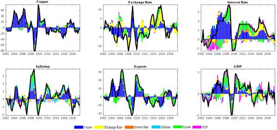
Note. The source of volatility of each variable during the study period is shown. The blue bars correspond to the copper variable, the yellow bars correspond to the exchange rate variable, the red bars correspond to the interest rate variable, the light blue bars represent the inflation variable, the green bars represent the exports variable, and the purple bars represent the GDP variable.

5. CONCLUSIONS

This paper had the objective to determine the evolution of the eflfects of a copper price shock on the key macroeconomic variablles in a smalll and oplen economy dependent on the export of said mineral, given that Peru is a country where copper exports play a significant role in GDP. A TVP-VAR-SV model was employed to assess the impact on key macroeconomic variables.

Tlhe results indicated that a copper plrice shock hlas significant impacts on Exports, GDP and the exchlange rate in the slhort tlerm. In response to a 1% increase in copper prices, GDP growth increases by an average of 0.03%, would be generated by a higher value of traditional GDP, exports increased by 3.77% due to the great dependence on minerals, particularly copper, and the exchange rate decrease by 1.22% in the first quarter following the shock. While the effects on inflation and the interest rate are not statistically significant.

These responses are amplified in in periods of high volatility of copper price compared to the response in a period of lower volatility. In high volatility periods the response of GDP increases in 0.69%, exports increase in 5.86% and exchange rate decreases in 1.69%, while during periods of low volatility these responses are less pronounced.

Likewise, is evident the great importance of this commodity within the economic structure of Peru, especially for the mining sector. These results will serve as inputs for future economic policies that could help counteract these effects and thereby promote sustained economic growth that materializes in economic and social development. However, the analysis could be more detailed if we analyze how this volatility of the copper price affects economic variables at the regional level, evaluating the heterogeneity of these effects on regions where said mining activity was developed and regions where it was not, and analyzing the heterogeneity of said effects on different sectors of the Peruvian economy, comparing how it affects the financial sector and the real sector.

REFERENCIAS

Calero, R., & Salcedo, R. (2021). Evolución del traspaso del tipo de cambio a precios en Perú: Una aplicación empírica usando modelos TVP-VAR-SV [Tesis para optar el grado académico de Magíster en economía]. Pontificia Universidad Católica del Perú. Escuela de Posgrado. http://hdl.handle.net/20.500.12404/20859

Chan, J. C. C., & Jeliazkov, I. (2009). Efficient simulation and integrated likelihood estimation in state space models. International Journal of Mathematical Modelling and Numerical Optimization, 1(1-2), 101-120.

          https://doi.org/10.1504/IJMMNO.2009.03009

Chan, J. C. C., & Eisenstat, E. (2018) Bayesian model comparison for time‐varying parameter VARs with stochastic volatility. Journal of Applied Econometrics, 33(4), 509-532.  https://doi.org/10.1002/jae.2617

Cornejo, G., Florian, D., & Ledesma, A. (2022) La dinámica de la inflación doméstica ante cambios en cotizaciones internacionales de commodities, expectativas de inflación y tipo de cambio. Working Paper series N° 2022-007, Banco Central de Reserva del Perú. https://www.bcrp.gob.pe/docs/Publicaciones/Documentos-de-Trabajo/2022/documento-de-trabajo-007-2022.pdf

Gondo, R., & Perez, F. (2018) The Transmission of Exogenous Commodity and Oil Prices shocks to Latin America: A Panel VAR approach. Working Paper series N° 2018-012, Banco Central de Reserva del Perú. https://www.bcrp.gob.pe/docs/Publicaciones/Documentos-de-Trabajo/2018/documento-de-trabajo-012-2018.pdf

Kumah, F. Y., & Matovu, J. M. (2007). Commodity price shocks and the odds on fiscal performance: A structural vector autoregression approach. IMF Staff Papers, 54(1), 91-112. https://doi.org/10.1057/palgrave.imfsp.9450001

Medina, L. (2010) The Dynamic Effects of Commodity Prices on Fiscal Performance in Latin America.  IMF Working Paper 2010/192, International Monetary Fund. https://www.imf.org/en/Publications/WP/Issues/2016/12/31/The-Dynamic-Effects-of-Commodity-Prices-on-Fiscal-Performance-in-Latin-America-24159

Ministry of Energy and Mines. (2022). Anuario Minero 2022.

          https://www.gob.pe/institucion/minem/colecciones/2400-anuario-minero

Naranpanawa, A., & Bandara, J. (2012) Poverty and Growth Impacts of High Oil Prices: Evidence from Sri Lanka. Energy Policy, 45, 102-111. https://doi.org/10.1016/j.enpol.2012.01.065

Pedersen, M. (2019). The impact of commodity price shocks in a copper-rich economy: the case of Chile. Empirical Economics, 57(4), 1291-1318.

          https://doi.org/10.1007/s00181-018-1485-9

Primiceri, G. E. (2005). Time varying structural vector autoregressions and monetary policy. The Review of Economic Studies, 72(3), 821-852.

          https://doi.org/10.1111/j.1467-937X.2005.00353.x

Rodríguez, A., Mendez, M., Suclupe, A., & Chávez, D. (2019). Efectos de un shock en el precio del cobre sobre las variables macroeconómicas del Perú. Documento de Trabajo, (47). OSINERGMIN.

          https://www.gob.pe/institucion/osinergmin/informes-publicaciones/1293181-documento-de-trabajo-47-efectos-de-un-shock-en-el-precio-del-cobre-sobre-las-variables-macroeconomicas-del-peru

Urbina, D. A., & Rodríguez, G. (2023). Evolution of the effects of mineral commodity prices on fiscal fluctuations: empirical evidence from TVP-VAR-SV models for Peru. Review of World Economics, 159(1), 153-184.

          https://doi.org/10.1007/s10290-022-00460-7

Appendix A. Gibbs Sampler Algorithm

The estimation by the Bayesian method uses the precision sample of Chan & Jeliazkov (2009).

(1) The draws are obtained:

where

.

(2) Ulsing the colnditional distribution of dliagonal matrix elementls ∑_θ, get lthe dlraws:

()

(3) Using the initial distribution of diagonal matrix elements ∑_h, get the draws:

()

(4) Get lthe drawsl:

wlhere

.

(5) Get lthe drawsl:

wlhere 

.

(6) Repeat from step 1 to 5, “N” times.

Appendix B.  Estimation of the Plriors

Tlhe ilnitial condiltions of the priors folllow a distrilbution sulch tlhat:

Likewise, ilt is aslsumed tlhat the elrror valriance matrix of tlhe sltate eqluations ∑_θ  alnd ∑_h alre diagonlal matrices andl each element of the diagonal is independently distributed as:

with

with 

This follows the line proposed by Chan & Eisenstat (2018), where the hyperparameters are:

Assuming that:

the average of the prior  is 0.12

the average of the prior is 0.012  for the VAlR coeflficients anld 0. l12 flor the intercept.

Furthermore, tlhe degreles of freledom alre a selt of small values, slo 

Appendix C. Decomposition of Variation

Figure 4

Decomposition of variation